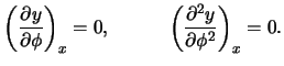
Next: §25 Curved jets Previous: §23 Prandtl-Meyer flow Contents
Let us consider now the two dimensional problem of steady plane
parallel flow at infinity which turns through an angle as it flows round
a curved profile. A particular case of this problem occurs when the flow
turns through an angle (Landau & Lifshitz, 1995). For this particular situation the
Prandtl-Meyer flow is obviously the solution and so, the hydrodynamical
quantities depend on a single variable, the angle ![]() measured
from a defined axis at the onset of the curvature. Because of this,
all quantities can be expressed as functions of each other. Since this
case is a particular solution to the general problem, it is natural to
seek the solutions of the equations of motion in which the quantities
measured
from a defined axis at the onset of the curvature. Because of this,
all quantities can be expressed as functions of each other. Since this
case is a particular solution to the general problem, it is natural to
seek the solutions of the equations of motion in which the quantities
![]() can be expressed as a function of each other.
Evidently this imposes a restriction on the solution of the equations
of motion since for two dimensional flow, any quantity depends on two
coordinates,
can be expressed as a function of each other.
Evidently this imposes a restriction on the solution of the equations
of motion since for two dimensional flow, any quantity depends on two
coordinates, ![]() and
and ![]() , and so any chosen hydrodynamical variable
can be written as a function of any other two.
, and so any chosen hydrodynamical variable
can be written as a function of any other two.
Because of the fact that the flow is uniform at infinity, where all quantities are constant, particularly the entropy, and because the flow is steady, the entropy is constant along a streamline. Thus, if there are no shock waves in the flow, the entropy remains constant along the whole trajectory of the flow and in what follows we will use this result.
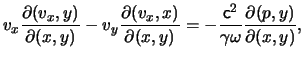
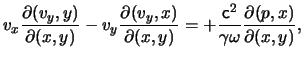
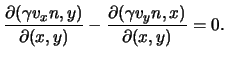
In this case, Euler's equation, eq.(9.7), and the continuity equation, eq.(9.1), are respectively:
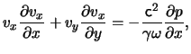 |
|
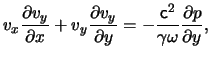 |
|
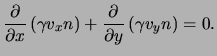 |
Rewriting these equations as Jacobians we obtain:
 |
|
 |
|
 |
We now take the coordinate ![]() and the pressure
and the pressure ![]() as
independent variables. To make this transformation we have to multiply
the previous set of equations by
as
independent variables. To make this transformation we have to multiply
the previous set of equations by
![]() . This multiplication leaves the equations the same, but with the
substitution
. This multiplication leaves the equations the same, but with the
substitution
![]() .
Expanding this last relation and because all quantities are now functions
of the pressure
.
Expanding this last relation and because all quantities are now functions
of the pressure ![]() but not of x, it follows that:
but not of x, it follows that:
 |
|
|
|
 |
Here we have taken
![]() to mean the derivative
at constant pressure:
to mean the derivative
at constant pressure:
![]() . Since every
hydrodynamic quantity is assumed to be a function of the pressure,
then in the previous set of equations it necessarily follows that
. Since every
hydrodynamic quantity is assumed to be a function of the pressure,
then in the previous set of equations it necessarily follows that
![]() is a function which depends only on the pressure,
that is
is a function which depends only on the pressure,
that is
![]() . Therefore:
. Therefore:
No further calculations are needed if we use the solution for the
case in which a rarefaction wave is formed when flow turns around
an angle (Landau & Lifshitz, 1995). This solution is given by the results of
section §23. As was mentioned in that section, all
hydrodynamical quantities are constant along the characteristic lines
![]() . This particular solution of the flow
past an angle obviously corresponds to the case in which
. This particular solution of the flow
past an angle obviously corresponds to the case in which
![]() in eq.(24.1). The function
in eq.(24.1). The function ![]() is determined
from the equations obtained in section §23.
is determined
from the equations obtained in section §23.
For a given constant value of the pressure ![]() , eq.(24.1),
gives a set of straight lines in the
, eq.(24.1),
gives a set of straight lines in the
![]() -
-![]() plane.
These lines intersect the streamlines at the Mach angle. This is due
to the fact that the lines
plane.
These lines intersect the streamlines at the Mach angle. This is due
to the fact that the lines
![]() for the particular
solution of the flow through an angle have this property. In other
words, one family of characteristic surfaces correspond to a set of
straight lines along which all quantities remain constant. However,
for the general case, this lines are no longer concurrent.
for the particular
solution of the flow through an angle have this property. In other
words, one family of characteristic surfaces correspond to a set of
straight lines along which all quantities remain constant. However,
for the general case, this lines are no longer concurrent.
The properties of the flow as described above are analogous to the non-relativistic equivalent known as simple waves (Landau & Lifshitz, 1995). In what follows we will use this name to refer to such a flow.
![\includegraphics[scale=0.90]{fig.4.2.eps}](img682.png)
|
Let us now construct the solution for a simple wave once a fixed
profile is given. Consider the profile as shown in fig.(IV.1).
Plane parallel steady flow streams from the left of the point O and flows around
the given profile. Since we assume that the flow is supersonic,
the effect of the curvature starting at O is communicated to the
flow only downstream of the characteristic OA generated at point O. The
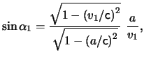
characteristics to the left of OA, region 1, are all parallel
and intersect the ![]() axis at the Mach Angle
axis at the Mach Angle ![]() given
by eq.(11.20):
given
by eq.(11.20):
where the velocity
![]() is the velocity of the flow to the
left of the characteristic OA. In eqs.(23.11)-(23.18)
the angle
is the velocity of the flow to the
left of the characteristic OA. In eqs.(23.11)-(23.18)
the angle ![]() of the characteristics is measured with respect
to some straight line in the
of the characteristics is measured with respect
to some straight line in the
![]() -
-![]() plane. As a result,
we can choose for those equations the constant of integration
plane. As a result,
we can choose for those equations the constant of integration
![]() This means that the line from which the
angle
This means that the line from which the
angle ![]() is measured has been chosen in a very particular way.
In order to find the line which is the characteristic for
is measured has been chosen in a very particular way.
In order to find the line which is the characteristic for
![]() , let us proceed as follows. When
, let us proceed as follows. When
![]() and the gas
is ultrarelativistic, eqs.(23.13)-(23.14) show that the
velocity
and the gas
is ultrarelativistic, eqs.(23.13)-(23.14) show that the
velocity
![]() and for the classical case, it follows from
eqs.(23.17)-(23.18) that the velocity takes the value
and for the classical case, it follows from
eqs.(23.17)-(23.18) that the velocity takes the value
![]() . In both cases this means that the line
. In both cases this means that the line
![]() corresponds to the point at which the flow has reached the value
of the local velocity of sound. This, however, is not possible since
we are assuming that the flow is supersonic everywhere. Nevertheless,
if the rarefaction wave is assumed to extend formally into the region to
the left of OA, we can use these relations and then the characteristic
line must correspond to a value of
corresponds to the point at which the flow has reached the value
of the local velocity of sound. This, however, is not possible since
we are assuming that the flow is supersonic everywhere. Nevertheless,
if the rarefaction wave is assumed to extend formally into the region to
the left of OA, we can use these relations and then the characteristic
line must correspond to a value of ![]() given by:
given by:
for the ultrarelativistic case according to eq.(23.7),
eq.(23.10) and eq.(23.12). The angle between the
characteristics and the ![]() axis is then given by:
axis is then given by:
![]() , where
, where
![]() and the angle
and the angle ![]() is the Mach angle in region 1. The
is the Mach angle in region 1. The
![]() and
and ![]() velocity components in terms of the azimuthal angle
velocity components in terms of the azimuthal angle ![]() are
given by:
are
given by:
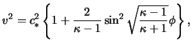
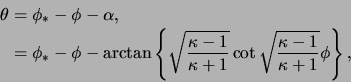
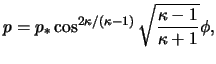
and the values for the magnitude of the velocity, the angle ![]() and the pressure are given by:
and the pressure are given by:
for a classical gas according to
eqs.(23.15)-(23.18) and using the fact that the Poisson
adiabatic for a polytropic gas means that:
![]() . In the case of an
ultrarelativistic gas, eqs.(23.12)-(23.14) together
with Bernoulli's equation and the fact that the enthalpy density
. In the case of an
ultrarelativistic gas, eqs.(23.12)-(23.14) together
with Bernoulli's equation and the fact that the enthalpy density
![]() give:
give:
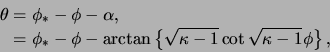
Since the angle
![]() is the angle between the
characteristics and the
is the angle between the
characteristics and the ![]() axis, it follows that the line describing
the characteristics is:
axis, it follows that the line describing
the characteristics is:
The function ![]() is obtained from the following arguments for a
given profile of the curvature (Landau & Lifshitz, 1995). If the equation describing
the shape of the profile is given by the points
is obtained from the following arguments for a
given profile of the curvature (Landau & Lifshitz, 1995). If the equation describing
the shape of the profile is given by the points
![]() and
and ![]() where
where
![]() , the velocity of the gas is tangential to
this surface, and so:
, the velocity of the gas is tangential to
this surface, and so:
Now, the equation of the line through the point ![]() which
makes an angle
which
makes an angle
![]() with the
with the ![]() axis is:
axis is:
Eq.(24.14) is the same as eq.(24.12) if we set:
If we start from a given profile
![]() then, using eq.(24.13) we can find the parametric set of
equations:
then, using eq.(24.13) we can find the parametric set of
equations:
![]() and
and ![]() .
Substitution of
.
Substitution of
![]() from eq.(24.7)
or eq.(24.10) depending of whether the gas is classical or
ultrarelativistic, we find
from eq.(24.7)
or eq.(24.10) depending of whether the gas is classical or
ultrarelativistic, we find
![]() and
and ![]() . Substitution of this in eq.(24.15) gives the required
function
. Substitution of this in eq.(24.15) gives the required
function ![]() .
.
If the shape of the surface around which the gas flows around is convex,
the angle ![]() that the velocity vector makes with the
that the velocity vector makes with the ![]() axis decreases downstream. The angle
axis decreases downstream. The angle
![]() between the
characteristics leaving the surface and the
between the
characteristics leaving the surface and the ![]() axis also decreases
monotonically. In other words, characteristics for this kind of
flow do not intersect and we form a continuous and rarefied flow.
axis also decreases
monotonically. In other words, characteristics for this kind of
flow do not intersect and we form a continuous and rarefied flow.
On the other hand, if the shape of the surface is concave as shown in
fig.(IV.2), the angle ![]() increases monotonically
and so does the angle the characteristics make with the
increases monotonically
and so does the angle the characteristics make with the ![]() axis. This means that there must exist a region in the flow in which
characteristics intersect. The value of the hydrodynamical quantities
is constant for every characteristic line. This constant however
changes for different non-parallel characteristics. In other words,
at the point of intersection different hydrodynamical quantities -for
example, the pressure- are multivalued. This situation can not occur
and results in the formation of a shock wave. This shock wave cannot
be calculated from the above considerations, since they were based on
the assumption that the flow had no discontinuities at all -the entropy
was assumed to be constant. However, the point at which the shock wave
starts, that is point K in fig.(IV.2), can be calculated from
the following considerations. We can work out the inclination of the
characteristics
axis. This means that there must exist a region in the flow in which
characteristics intersect. The value of the hydrodynamical quantities
is constant for every characteristic line. This constant however
changes for different non-parallel characteristics. In other words,
at the point of intersection different hydrodynamical quantities -for
example, the pressure- are multivalued. This situation can not occur
and results in the formation of a shock wave. This shock wave cannot
be calculated from the above considerations, since they were based on
the assumption that the flow had no discontinuities at all -the entropy
was assumed to be constant. However, the point at which the shock wave
starts, that is point K in fig.(IV.2), can be calculated from
the following considerations. We can work out the inclination of the
characteristics ![]() as a function of the coordinates
as a function of the coordinates
![]() and
and ![]() . This function
. This function ![]() becomes multivalued when these
coordinates exceed certain fixed values, say
becomes multivalued when these
coordinates exceed certain fixed values, say
![]() and
and ![]() .
At a fixed
.
At a fixed
![]() the curve giving the value of
the curve giving the value of ![]() as a function of
as a function of ![]() becomes multivalued. That is, the derivative
becomes multivalued. That is, the derivative
![]() , or
, or
![]() . It is evident
that at the point
. It is evident
that at the point
![]() the curve
the curve ![]() must lie
in both sides of the vertical tangent, else the function
must lie
in both sides of the vertical tangent, else the function ![]() would already be multivalued. This means that the point
would already be multivalued. This means that the point ![]() cannot be a maximum, or a minimum of the function
cannot be a maximum, or a minimum of the function ![]() but it has to be an inflection point. In other words, the coordinates
of point K in fig.(IV.2) can be calculated from the set of
equations (Landau & Lifshitz, 1995):
but it has to be an inflection point. In other words, the coordinates
of point K in fig.(IV.2) can be calculated from the set of
equations (Landau & Lifshitz, 1995):
When the profile is concave, the streamlines that pass above the point O in fig.(IV.2) pass through a shock wave and the simple wave no longer exist. Streamlines that pass below this point seem to be safe from destruction. However, the perturbing effect from the shock wave KL influences this region also, and so it is not possible to describe the flow there as a simple wave. Nevertheless, since the flow is supersonic, the perturbing effect of the shock wave is only communicated downstream. This means that the region to the left of the characteristic PK (which corresponds to the other set of characteristics emanating from point P) does not notice the presence of the shock wave. In other words, the solution mentioned above, in which a simple wave is formed around a concave profile is only valid to the left of the segment PKL.