Next: §12 Polytropic gases Previous: §10 Classical equations of Contents
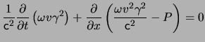
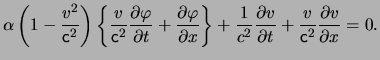
Let us consider now the one dimensional problem of a relativistic flow
in which dissipation processes are not taken into account, that is, the
entropy remains constant as the fluid moves. For this particular case,
the continuity equation, eq.(9.1) and the ![]() -component of
the equations of motion, eq.(8.1) are given by:
-component of
the equations of motion, eq.(8.1) are given by:
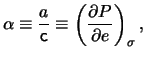
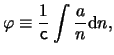
respectively. If we define the quantities:
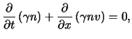
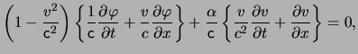
then eq.(11.1) and eq.(11.2) can be written as:
Addition and substraction of these two relations gives:
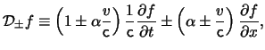
for any function ![]() . From the definitions of the
operator
. From the definitions of the
operator ![]() in eq.(11.8), it follows that:
in eq.(11.8), it follows that:
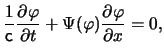
and hence, eqs.(11.7) become:
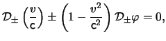
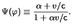
If we now introduce the parameters:
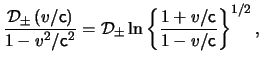
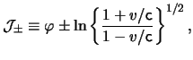
which are called Riemann invariants, then eqs.(11.9), that is, eqs.(11.1)-(11.2), become equivalent to (Taub, 1948; Taub, 1978):
From this relation it follows that the Riemann invariants
![]() are constant along the curves
are constant along the curves
![]() respectively. These curves
respectively. These curves
![]() are called characteristics and play an essential role in fluid
dynamics. The differential operators that appear inside the brackets
in eq.(11.11) are the operators of differentiation along the
characteristics
are called characteristics and play an essential role in fluid
dynamics. The differential operators that appear inside the brackets
in eq.(11.11) are the operators of differentiation along the
characteristics
![]() in the
in the
![]() -
-![]() plane.
plane.
In general terms, a disturbance is said to propagate as a
travelling wave (Taub, 1948; Landau & Lifshitz, 1995) if either
![]() or
or ![]() is constant. For instance, consider the
case in which
is constant. For instance, consider the
case in which
![]() , then from
eq.(11.10), and eq.(11.11) it follows that (Taub, 1948):
, then from
eq.(11.10), and eq.(11.11) it follows that (Taub, 1948):
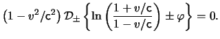
The general solution of eq.(11.12) is
in which
![]() is an arbitrary function.
The relation eq.(11.14) means that
is an arbitrary function.
The relation eq.(11.14) means that ![]() is constant
along straight lines with slope
is constant
along straight lines with slope
![]() in the plane
in the plane
![]() -
-![]() . In other words,
. In other words,
![]() is the
velocity of propagation of
is the
velocity of propagation of ![]() . From the definition of
. From the definition of ![]() in eq.(11.13) it follows that, for weak disturbances in which
in eq.(11.13) it follows that, for weak disturbances in which
![]() then
then ![]() .
.
The speed of sound is the velocity at which adiabatic perturbations
of small amplitude in a compressible fluid move with respect to the
flow. Due to the fact that
![]() as
as ![]() , it is obvious that
, it is obvious that ![]() represents
the speed of sound in units of the speed of light
represents
the speed of sound in units of the speed of light![]() .
.
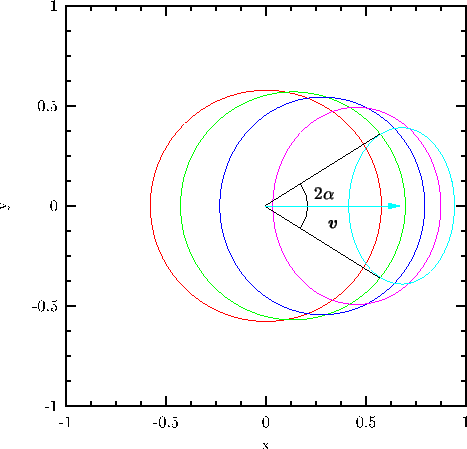
The properties of subsonic and supersonic flow, that is flow with velocity less or greater than that of sound, are completely different in nature. To begin with, let us see how perturbations with small amplitudes are propagated along the flow for both, subsonic and supersonic flows. For simplicity in the following discussion we will consider two dimensional flow only. The relations obtained below are easily generalised for the general case of three dimensions.
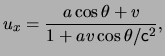
If a gas in a steady motion receives a small perturbation, this
propagates through the gas with the velocity of sound relative to the
flow itself. In another system of reference, the laboratory frame,
in which the velocity of the flow is
![]() along the
along the ![]() axis,
the perturbation travels with an observed velocity
axis,
the perturbation travels with an observed velocity
![]() whose
whose
![]() and
and ![]() components are given by:
components are given by:
according to the rule for the addition of velocities in
special relativity (Landau & Lifshitz, 1994a). The polar angle ![]() and the velocity of sound
and the velocity of sound ![]() are both measured in the proper frame
of the fluid. Since a small disturbance in the flow moves with
the velocity of sound in all directions, the parameter
are both measured in the proper frame
of the fluid. Since a small disturbance in the flow moves with
the velocity of sound in all directions, the parameter ![]() can have values
can have values
![]() . This is
illustrated pictorially in fig.(II.1).
. This is
illustrated pictorially in fig.(II.1).
![\includegraphics[scale=0.70]{fig.2.1.eps}](img259.png)
|
Let us consider first the case in which the flow is subsonic,
as is presented in case (a) of fig.(II.1). Since by
definition
![]() and
and
![]() , it follows
from eqs.(11.15)-(11.16) that
, it follows
from eqs.(11.15)-(11.16) that
![]() while
while ![]() .
In other words, the region influenced by the perturbation contains the
velocity vector
.
In other words, the region influenced by the perturbation contains the
velocity vector
![]() . This means that the perturbation
originating at
. This means that the perturbation
originating at ![]() is able to be transmitted to all the flow.
is able to be transmitted to all the flow.
When the velocity of the flow is supersonic, the situation is quite
different, as shown in case (b) of fig.(II.1). For this case
it follows that
![]() and
and ![]() . In other words, the velocity
vector
. In other words, the velocity
vector
![]() is not fully contained inside the region of
influence produced by the perturbation. This implies that only a bounded
region of space will be influenced by the perturbation originated at
position
is not fully contained inside the region of
influence produced by the perturbation. This implies that only a bounded
region of space will be influenced by the perturbation originated at
position ![]() . For the case of steady flow, this region is evidently
a cone. Thus, a disturbance arising at any point in supersonic flow
is propagated only downstream inside a cone of aperture angle
. For the case of steady flow, this region is evidently
a cone. Thus, a disturbance arising at any point in supersonic flow
is propagated only downstream inside a cone of aperture angle ![]() . By definition, the angle
. By definition, the angle ![]() is such that it is
the angle subtended by the unit radius vector
is such that it is
the angle subtended by the unit radius vector
![]() with the velocity vector
with the velocity vector
![]() at the point in
which the azimuthal unit vector
at the point in
which the azimuthal unit vector
![]() is
orthogonal with the tangent vector
is
orthogonal with the tangent vector
![]() to the boundary of the region influenced
by the perturbation. The unit vector
to the boundary of the region influenced
by the perturbation. The unit vector
![]() is the unit radial vector in the proper frame of the flow. In other
words, the angle
is the unit radial vector in the proper frame of the flow. In other
words, the angle ![]() obeys the following mathematical relation:
obeys the following mathematical relation:
Substitution of eqs.(11.15)-(11.16) into eq.(11.17) gives:
On the other hand, since
![]() ,
it follows from eqs.(11.15)-(11.16) and eq.(11.18)
that:
,
it follows from eqs.(11.15)-(11.16) and eq.(11.18)
that:
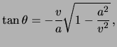
so eq.(11.18) gives a relation between the angle ![]() , the velocity of the flow
, the velocity of the flow
![]() and its sound speed
and its sound speed ![]() :
:
This variation of the angle ![]() is plotted in
fig.(II.2) for the case in which the gas is assumed to have
a relativistic equation of state, that is, when
is plotted in
fig.(II.2) for the case in which the gas is assumed to have
a relativistic equation of state, that is, when
![]() .
The important feature to note from the plot is that the aperture angle of
the cone of influence is reduced when the velocity of the flow approaches
that of light.
.
The important feature to note from the plot is that the aperture angle of
the cone of influence is reduced when the velocity of the flow approaches
that of light.
From eq.(11.19) it follows that, as the velocity of the
flow approaches that of light, the angle ![]() vanishes.
In other words, as the velocity reaches its maximum possible value, the
perturbation is communicated in a very narrow region along the velocity
of the flow.
vanishes.
In other words, as the velocity reaches its maximum possible value, the
perturbation is communicated in a very narrow region along the velocity
of the flow.
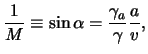
In studies of supersonic motion of fluid mechanics it is very useful
to introduce a dimensionless quantity ![]() defined as:
defined as:
according to eq.(11.19). The quantity
![]() is the Lorentz factor
for the velocity of sound
is the Lorentz factor
for the velocity of sound ![]() . The number
. The number ![]() has the
property that
has the
property that
![]() as
as ![]() and
and ![]() as
as ![]() . It also follows that
. It also follows that
![]() if and only if
if and only if
![]() .
.
|
The surface bounding the region reached by a disturbance starting
from the origin ![]() is called a characteristic surface
(Landau & Lifshitz, 1995). This definition of characteristic and that given above,
when the Riemann invariants were introduced, are the same in the sense
that the characteristics introduced here are curves in the
is called a characteristic surface
(Landau & Lifshitz, 1995). This definition of characteristic and that given above,
when the Riemann invariants were introduced, are the same in the sense
that the characteristics introduced here are curves in the
![]() -
-![]() plane which cut the streamlines in this plane at the Mach angle.
Those discussed above correspond to curves in the
plane which cut the streamlines in this plane at the Mach angle.
Those discussed above correspond to curves in the
![]() -
-![]() plane which cut the streamlines (that is, the curves
plane which cut the streamlines (that is, the curves ![]() for which
for which
![]() ) at the Mach
angle in this plane.
) at the Mach
angle in this plane.
In the general case of arbitrary steady flow, the characteristic
surface is no longer a cone. However, exactly as it was shown above,
the characteristic surface cuts the streamlines at any point at the
angle ![]() .
.
One of the main differences between supersonic and subsonic flow
is the possibility of a certain type of discontinuities in the flow,
called shock waves. For example, from eq.(11.14)
it follows that for certain functions
![]() , which are
determined by the particular boundary conditions of the problem in
question, the curves
, which are
determined by the particular boundary conditions of the problem in
question, the curves
![]() in the
in the
![]() -
-![]() plane intersect. Since the Riemann invariants as defined
in eq.(11.10) are constant along these curves, with a different
constant for each curve, it follows that for travelling waves the velocity
plane intersect. Since the Riemann invariants as defined
in eq.(11.10) are constant along these curves, with a different
constant for each curve, it follows that for travelling waves the velocity
![]() and the other hydrodynamical variables are multivalued. This is
impossible in any physical circumstance and results in the creation of
strong discontinuities (shock waves) on the flow.
and the other hydrodynamical variables are multivalued. This is
impossible in any physical circumstance and results in the creation of
strong discontinuities (shock waves) on the flow.
Let us briefly discuss the classical limit of the different physical
circumstances mentioned above. To do this, we make use of the relations
presented in eq.(10.1) with
![]() and, as it is usual in the classical case, we represent the speed of
sound by
and, as it is usual in the classical case, we represent the speed of
sound by ![]() .
.
First of all, the speed of sound ![]() is:
is:
The Riemann invariants
![]() are constant along
the curves
are constant along
the curves
![]() .
The dimensionless number
.
The dimensionless number ![]() satisfies the following relation:
satisfies the following relation:
and is called in classical hydrodynamics the Mach
number.![]()
The results obtained about the relativistic and classical Mach number ![]() can be rewritten in the following way:
can be rewritten in the following way:
As a way to compare the difference between the classical and relativistic Mach numbers, a plot of both of them is presented in fig.(II.3). The intersection of both curves occurs for the case in which the Mach number tends to unity, that is when the velocity of the flows tend to the local velocity of sound according to Theorem 1. For the case of subsonic flow, the relativistic Mach number is less than its classical counterpart. However for supersonic flow the relativistic Mach number is greater than the classical one.
![\includegraphics[scale=0.80]{fig.2.3.eps}](img300.png)
|
![$\displaystyle \left[ \left( 1 \pm \alpha \frac{ \ensuremath{v}}{ \ensuremath{\m...
...athsf{c}}} \right) \frac{ \partial }{ \partial x } \right] \mathcal{J}_\pm = 0.$](img235.png)
![$\displaystyle \frac{ 1 }{ M } = \sin{\alpha} \xrightarrow[\ensuremath{\mathsf{c}}\rightarrow \infty]{} \frac{ \ensuremath{v}}{ c }$](img296.png)