Next: §14 One-dimensional similarity flow Previous: §12 Polytropic gases Contents
One of the most important physical phenomena that occur in supersonic
flow is the existence of discontinuities in the different hydrodynamical
quantities describing the flow. In order for the flow to possess
such discontinuities, certain conditions have to be satisfied at the
boundaries between the media. Mathematically, these boundaries are
treated as infinitesimal, so that they may be assumed to be surfaces.
For a steady flow, an element of area on a surface of discontinuity
can be considered to be a plane and it can be assumed to be at rest by
an appropriate choice of the system of reference. If the flow is not
steady, then the argument remains valid for a short interval of time.
In order to simplify the calculations, and without loss of generality, the
surface of discontinuity can be chosen to be a plane which is parallel to
the ![]() plane, so that the unit vector
plane, so that the unit vector
![]() in the positive
in the positive ![]() direction is normal to it.
direction is normal to it.
Let us consider a closed three dimensional timelike cylinder ![]() that intersects the surface of discontinuity. The axis of the cylinder
is such that it is parallel to the normal to the plane of the surface
of discontinuity, in the direction of the
that intersects the surface of discontinuity. The axis of the cylinder
is such that it is parallel to the normal to the plane of the surface
of discontinuity, in the direction of the ![]() axis. Integrating
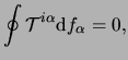
eq.(8.1) and eq.(9.1) along the volume enclosed by
this hypersurface and using Gauss's theorem we obtain:
axis. Integrating
eq.(8.1) and eq.(9.1) along the volume enclosed by
this hypersurface and using Gauss's theorem we obtain:
with
![]() the area element along the
surface
the area element along the
surface ![]() . Taking the limit when the volume enclosed by the area
. Taking the limit when the volume enclosed by the area ![]() tends to zero gives:
tends to zero gives:
where the difference between the values on either side
of the discontinuity (sides 1 and 2) are represented by
![]() for any quantity
for any quantity ![]() . As we saw in section
§8,
. As we saw in section
§8,
![]() represents
the energy flux vector,
represents
the energy flux vector,
![]() is the 3-momentum flux density vector and
is the 3-momentum flux density vector and ![]() is the
particle flux 4-vector. From this it follows that the particle flux,
the energy flux and the momentum flux vectors are conserved across the
surface of discontinuity according to eq.(13.3):
is the
particle flux 4-vector. From this it follows that the particle flux,
the energy flux and the momentum flux vectors are conserved across the
surface of discontinuity according to eq.(13.3):
|
and
| |
| (13.4) | |
where
![]() and
and ![]() are Cartesian coordinates.
From eqs.(13.4)-(13.5) it follows that it is possible
to define two types of discontinuities. In the first place, those in
which there is no particle flux through the surface of discontinuity.
That is,
are Cartesian coordinates.
From eqs.(13.4)-(13.5) it follows that it is possible
to define two types of discontinuities. In the first place, those in
which there is no particle flux through the surface of discontinuity.
That is,
![]() . Since the particle number
densities on both sides of the discontinuity are non-zero it follows
that the velocities
. Since the particle number
densities on both sides of the discontinuity are non-zero it follows
that the velocities
![]() . This satisfies identically
all relations in eq.(13.5) as well as the first and third of
eq.(13.4). The second relation in eq.(13.4) implies
. This satisfies identically
all relations in eq.(13.5) as well as the first and third of
eq.(13.4). The second relation in eq.(13.4) implies
![]() . That is, a discontinuity for which the mass flux through
its surface is zero is such that its normal velocity components are zero
and the pressure is continuous across it:
. That is, a discontinuity for which the mass flux through
its surface is zero is such that its normal velocity components are zero
and the pressure is continuous across it:
The values of the other hydrodynamical quantities can take
any value across this surface of discontinuity. A discontinuity of this
kind is called a tangential discontinuity.![]()
The second type of discontinuity occur when the particle flux through the surface is non-zero. According to eqs.(13.4)-(13.5), this implies that the tangential component of the velocity is preserved across the surface of discontinuity:
Such discontinuities are called shock waves. Substitution of the 4-velocity components in eq.(13.4) gives:
in which
![]() is the
proper volume per particle number. From eq.(13.8) and
eq.(13.10) it follows that the particle number flux
is the
proper volume per particle number. From eq.(13.8) and
eq.(13.10) it follows that the particle number flux ![]() is given by:
is given by:
Algebraic manipulation of eqs.(13.8)-(13.10) imply that (Taub, 1948; Landau & Lifshitz, 1995):
which is called the relativistic shock adiabatic relation
or Taub adiabatic. For a given
![]() , the shock
adiabatic gives a relation between
, the shock
adiabatic gives a relation between
![]() .
.
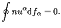
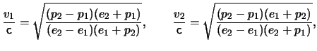
Writing
![]() so that
so that ![]() , the velocities of the gas on either side of the
discontinuity can be easily shown to be:
, the velocities of the gas on either side of the
discontinuity can be easily shown to be:
according to the relativistic rule for addition of velocities.
The entropy density, as any other thermodynamic quantity, is discontinuous
across a shock wave. From the law of the increase of the entropy it
follows that the entropy can only increase across a shock wave. It is
possible to show under very general arguments (Thorne, 1973; Landau & Lifshitz, 1995)
that the shock wave is a compression wave, that is
![]() , if
, if
When
![]() it follows from
eqs.(13.8)-(13.10) that
it follows from
eqs.(13.8)-(13.10) that
![]() . Using the definition of the particle number flux in
eq.(13.8), this implies that
. Using the definition of the particle number flux in
eq.(13.8), this implies that
![]() . In other
words, provided that the inequality in eq.(13.15) is satisfied,
then a shock wave satisfies:
. In other
words, provided that the inequality in eq.(13.15) is satisfied,
then a shock wave satisfies:
Very general arguments about the stability of shock waves (Landau & Lifshitz, 1995) show that, for any shock wave, whatever the thermodynamic conditions of the gas:
for a gas with sound speed ![]() .
.
In order to derive the classical expressions of the relations written
above, we take the limit
![]() and
use eq.(10.1). It is common practice in classical hydrodynamics to
use the mass flux density
and
use eq.(10.1). It is common practice in classical hydrodynamics to
use the mass flux density ![]() as opposed to the particle number density
as opposed to the particle number density
![]() , and the inverse of the mass density, the volume per unit
mass
, and the inverse of the mass density, the volume per unit
mass
![]() , instead of the volume per unit particle
, instead of the volume per unit particle
![]() .
.
The mass density flux ![]() is then given by:
is then given by:
The shock adiabatic relation, also called Hugoniot adiabatic in classical fluid dynamics, is:
The velocity difference in eq.(13.14) gives:
All the inequalities in eqs.(13.16)-(13.17)
remain valid and that in eq.(13.15) becomes
![]() .
.