Next: III Jet-cloud interactions: bent Previous: §13 Shock waves in Contents
In this section we will discuss the one-dimensional non-steady gas flow under the assumption that there are characteristic velocities in the flow, but not characteristic lengths. To simplify the discussion we assume that relativistic effects are not taken into account.
The state of the flow at any time is defined by the characteristic
velocity parameter and by some other parameters which describe the state
of the gas, for example the pressure and density at an initial instant.
With these parameters alone it is not possible to find a combination
which has the dimensions of length or time. By applying the ![]() -Theorem of dimensional analysis (Sedov, 1993) it follows that the
distribution of the different hydrodynamical quantities can only depend
on the position
-Theorem of dimensional analysis (Sedov, 1993) it follows that the
distribution of the different hydrodynamical quantities can only depend
on the position ![]() and time
and time ![]() through the ratio
through the ratio
![]() only. In other words, if the lengths are measured in
a unit that increases proportional with time, the pattern produced by
the flow remains unchanged. Such a flow is called a similarity
flow (Landau & Lifshitz, 1995).
only. In other words, if the lengths are measured in
a unit that increases proportional with time, the pattern produced by
the flow remains unchanged. Such a flow is called a similarity
flow (Landau & Lifshitz, 1995).
Using the fact that all quantities in the problem depend only on the
single variable ![]() , for which
, for which
![]() and
and ![]() , we obtain from the equation
of conservation of the entropy, eq.(10.4),
, we obtain from the equation
of conservation of the entropy, eq.(10.4),
![]() . The prime denotes differentiation with respect to
. The prime denotes differentiation with respect to ![]() .
From this equation it follows that
.
From this equation it follows that
![]() , otherwise as it
is obvious from the equations presented below in eq.(14.1) a
contradiction will be obtained. This implies that the entropy
, otherwise as it
is obvious from the equations presented below in eq.(14.1) a
contradiction will be obtained. This implies that the entropy
![]() const
const![]() and so, similarity flow in one dimension which is
adiabatic must also be isentropic. In exactly the same way, the
and so, similarity flow in one dimension which is
adiabatic must also be isentropic. In exactly the same way, the
![]() and
and ![]() components of Euler's equation imply that the velocity
in the
components of Euler's equation imply that the velocity
in the
![]() and
and ![]() components are constant and we can take them
as zero by an appropriate choice of the system of reference.
components are constant and we can take them
as zero by an appropriate choice of the system of reference.
The ![]() component of Euler's equation, eq.(10.3), and
the continuity equation eq.(10.2) can be written as:
component of Euler's equation, eq.(10.3), and
the continuity equation eq.(10.2) can be written as:
Here
![]() denotes the velocity in the
denotes the velocity in the ![]() direction
and we will use that convention in what follows. The trivial solution of
this last set of equations is that of a uniform flow with
direction
and we will use that convention in what follows. The trivial solution of
this last set of equations is that of a uniform flow with
![]() const
const![]() const
const![]() . The non-trivial solution is
found by eliminating
. The non-trivial solution is
found by eliminating
![]() and
and ![]() from the equations,
giving
from the equations,
giving
![]() , so that
, so that
![]() .
We take the plus sign in the following discussion, which means that we
have taken the direction of the positive
.
We take the plus sign in the following discussion, which means that we
have taken the direction of the positive ![]() axis in a definite manner:
axis in a definite manner:
Substituting eq.(14.3) into eq.(14.1) we obtain
![]() . In order to integrate this
relation we recall that the velocity of sound is a function of the
thermodynamical state of the gas. We can thus take this velocity as
a function of the entropy and the mass density. Since the entropy is
constant it follows that the velocity of sound can be considered as a
function of the density only. In other words (Landau & Lifshitz, 1995):
. In order to integrate this
relation we recall that the velocity of sound is a function of the
thermodynamical state of the gas. We can thus take this velocity as
a function of the entropy and the mass density. Since the entropy is
constant it follows that the velocity of sound can be considered as a
function of the density only. In other words (Landau & Lifshitz, 1995):
where the choice of the independent variable remains open.
Let us briefly discuss some general properties of the solution.
Differentiating eq.(14.3) with respect to ![]() gives:
gives:
 |
(14.6) |
|
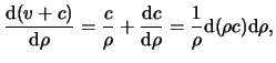
The derivative of tex2html_wrap_inline tex2html_wrap_inlinev+ c can be calculated from eq.(14.4) which gives:
| |
 |
|
|
and
| |
|
Differentiation of this relation results in:
| |
|
so that eq.(14.6) takes the form:
| |
| (14.7) | |
Substitution of eq.(14.7) into eq.(14.6)
implies that
![]() for
for ![]() .
Because
.
Because
![]() , it
follows that
, it
follows that
![]() . Also, since
. Also, since
![]() according
to eq.(14.4), the inequality
according
to eq.(14.4), the inequality
![]() holds. In other words, we have proved that the following relations
are valid in a flow for which eq.(14.3) holds:
holds. In other words, we have proved that the following relations
are valid in a flow for which eq.(14.3) holds:
In order to understand the meaning of these inequalities, let us rewrite
them not as variations of the position ![]() but as variations of the
of time for a given fluid element as it moves. This variation is given
by the total derivative of the corresponding quantity with respect to
time. Thus, for the density it follows from the equation of continuity
and eq.(14.8) that:
but as variations of the
of time for a given fluid element as it moves. This variation is given
by the total derivative of the corresponding quantity with respect to
time. Thus, for the density it follows from the equation of continuity
and eq.(14.8) that:
![]() . This implies that
. This implies that
![]() also. On the other hand,
Euler's equation implies that
also. On the other hand,
Euler's equation implies that
![]() .
It is important to note that this last inequality does not mean that the
magnitude of the velocity decreases as the fluid moves about, since
.
It is important to note that this last inequality does not mean that the
magnitude of the velocity decreases as the fluid moves about, since
![]() can be negative. We have proved that, as the fluid moves, the
following inequalities are satisfied:
can be negative. We have proved that, as the fluid moves, the
following inequalities are satisfied:
This means that, as the fluid moves, its pressure and density decreases. To put it differently, the gas is continuously rarefied as the fluid moves. Such a flow is called a rarefaction wave.
A rarefaction wave can only be propagated a finite distance along the ![]() axis. This follows from the fact that
axis. This follows from the fact that
![]() as
as ![]() . As a result, we can apply
eq.(14.3) at the boundaries of a rarefaction wave. For this
case, the ratio
. As a result, we can apply
eq.(14.3) at the boundaries of a rarefaction wave. For this
case, the ratio ![]() is the velocity of the boundary relative to
a fixed system of coordinates. The velocity relative to the flow itself
is
is the velocity of the boundary relative to
a fixed system of coordinates. The velocity relative to the flow itself
is
![]() which is equal to the local velocity of sound
which is equal to the local velocity of sound ![]() according to eq.(14.3). This result implies that the boundaries
of a rarefaction wave are weak discontinuities.
according to eq.(14.3). This result implies that the boundaries
of a rarefaction wave are weak discontinuities.![]()
The choice of sign in eq.(14.3) is now clear. It must be such
that the weak discontinuities, bounding the rarefaction wave, are assumed
to be moving in the positive ![]() direction relative to the gas.
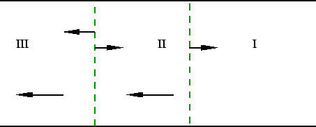
By an appropriate choice of the system of reference we can choose the
region, region I, to the right of the rarefaction wave to be at rest,
as it is shown in fig.(II.4). Region II is the rarefaction
wave and region III has gas moving with constant velocity. The arrows
in the figure represent the direction of the flow and of the weak
discontinuities. Due to the fact that the weak discontinuities move
to the right relative to the gas, the weak discontinuity at the right
of the diagram moves to the right. However, the weak discontinuity on
the left might move in either direction. The direction depends on the
value of the velocity reached in the rarefaction wave (Landau & Lifshitz, 1995).
direction relative to the gas.
By an appropriate choice of the system of reference we can choose the
region, region I, to the right of the rarefaction wave to be at rest,
as it is shown in fig.(II.4). Region II is the rarefaction
wave and region III has gas moving with constant velocity. The arrows
in the figure represent the direction of the flow and of the weak
discontinuities. Due to the fact that the weak discontinuities move
to the right relative to the gas, the weak discontinuity at the right
of the diagram moves to the right. However, the weak discontinuity on
the left might move in either direction. The direction depends on the
value of the velocity reached in the rarefaction wave (Landau & Lifshitz, 1995).
|
For a polytropic gas eq.(14.4) gives:
in which the constant of integration ![]() corresponds to the
value of the velocity of sound when the velocity of the rarefaction wave
vanishes. Here and in what follows we denote by the suffix
corresponds to the
value of the velocity of sound when the velocity of the rarefaction wave
vanishes. Here and in what follows we denote by the suffix ![]() the
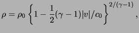
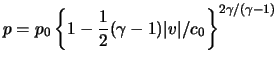
region of the flow where the gas is at rest. Using the Poisson adiabatic
for a polytropic gas, and rewriting eq.(14.10), we find that:
the
region of the flow where the gas is at rest. Using the Poisson adiabatic
for a polytropic gas, and rewriting eq.(14.10), we find that:
 |
(14.11) |
 |
(14.12) |
 |
(14.13) |
|
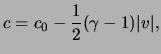
The value of the velocity as a function of the ratio tex2html_wrap_inline x / t is obtained by substituting eq.(14.11) in eq.(14.3):
| |
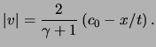 |
(14.14) |
Lastly we mention that from eq.(14.11), since the velocity of sound is non negative, the following inequality has to be satisfied:
When the velocity reaches this limiting value, the pressure,
density and velocity of sound in the gas become zero.