Next: §18 Isothermal cloud Previous: §16 Initial stages of Contents
Once the steady state is reached, the jet penetrates the cloud and expands adiabatically. Because of this, the trajectory of the jet is determined by Euler's equation, eq.(10.6), which can be written as:
where
![]() and
and![]() represent the
heat function per unit mass and the velocity of the flow inside the jet.
The gravitational forces produced by the mass of the cloud in the moving
jet is given by the gradients of the gravitational potential
represent the
heat function per unit mass and the velocity of the flow inside the jet.
The gravitational forces produced by the mass of the cloud in the moving
jet is given by the gradients of the gravitational potential ![]() .
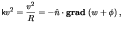
The curvature
.
The curvature
![]() of the trajectory appears in the term
which is proportional to its normal direction
of the trajectory appears in the term
which is proportional to its normal direction
![]() .
These two terms are proportional to the gradients of the unit tangent
vector
.
These two terms are proportional to the gradients of the unit tangent
vector
![]() in the following way:
in the following way:
![]() . From eq.(17.1)
there are two equivalent ways of finding the required trajectory. The first
is due to Icke (1991) and is as follows. Multiplying
eq.(17.1) by the normal unit vector
. From eq.(17.1)
there are two equivalent ways of finding the required trajectory. The first
is due to Icke (1991) and is as follows. Multiplying
eq.(17.1) by the normal unit vector
![]() to the jet trajectory one finds:
to the jet trajectory one finds:
where ![]() is the radius of curvature to the trajectory.
Eq.(17.2) simply means that the normal components of the gradients
of the pressure in the jet (right hand side of that equation) have to
balance the centrifugal acceleration produced by the curvature of
the jet (left hand side of that equation).
is the radius of curvature to the trajectory.
Eq.(17.2) simply means that the normal components of the gradients
of the pressure in the jet (right hand side of that equation) have to
balance the centrifugal acceleration produced by the curvature of
the jet (left hand side of that equation).
The second method used to find the trajectory to the jet is due
to Cantó & Raga (1996) and Raga & Cantó (1996). Instead of performing scalar
multiplication of eq.(17.1) with a normal vector, contraction
is carried out with a tangent vector
![]() .
This implies that
.
This implies that
![]() , that is, the
path of the jet is described by Bernoulli's theorem eq.(10.7).
, that is, the
path of the jet is described by Bernoulli's theorem eq.(10.7).
It is straightforward to show that if the flow in the jet is irrotational (as it is for the case we are going to consider, according to the results presented below), both relations, eq.(17.2) and Bernoulli's law are equivalent. For, if the vorticity is zero, then from the relation:
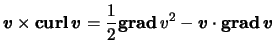
combined with Euler's equation, it follows that
![]() , which is a particular form of Bernoulli's law. Multiplication of
this relation by the normal unit vector
, which is a particular form of Bernoulli's law. Multiplication of
this relation by the normal unit vector
![]() gives eq.(17.2). Since it is natural to work with energies,
the approach by (1996) and (1996) will be used in
what follows.
gives eq.(17.2). Since it is natural to work with energies,
the approach by (1996) and (1996) will be used in
what follows.
Let us show now that under the conditions we have previously described,
the trajectory of the jet is two dimensional. From Euler's equation,
it follows that the left hand side of eq.(10.6) is simply
the force per unit mass experienced by a fluid particle as it moves.
Since all quantities in the right hand side of that equation depend only
on the distance from the cloud's centre ![]() , vector multiplication of
the radius vector
, vector multiplication of
the radius vector
![]() with eq.(10.6) implies
with eq.(10.6) implies
![]() . In other words, the specific angular momentum
. In other words, the specific angular momentum
![]() is conserved as the fluid moves. Since the radius vector is perpendicular
to the angular momentum vector, the motion is two dimensional, and so,
polar coordinates
is conserved as the fluid moves. Since the radius vector is perpendicular
to the angular momentum vector, the motion is two dimensional, and so,
polar coordinates
![]() are used in the
following analysis.
are used in the
following analysis.
Consider a situation in which the jet enters the cloud parallel to
the ![]() axis at a distance
axis at a distance ![]() , so that its velocity vector
is initially given by:
, so that its velocity vector
is initially given by:
where
![]() ,
,
![]() and
and
![]() are unit vectors in the directions
are unit vectors in the directions ![]() ,
, ![]() and
and ![]() respectively. Because angular momentum is conserved
and the motion is two dimensional, the velocity is most simply written
using eq.(17.3) as:
respectively. Because angular momentum is conserved
and the motion is two dimensional, the velocity is most simply written
using eq.(17.3) as:
in which
![]() represents
the velocity in the radial direction.
represents
the velocity in the radial direction.
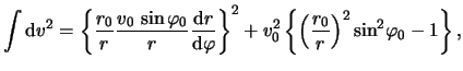
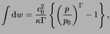
Since the steady flow of the jet expands adiabatically, we can calculate the path of the jet by means of Bernoulli's equation, eq.(10.7):
in which the line integrals are taken from the initial position
of a given fluid particle. The heat function per unit mass ![]() of the
flow in the jet is given by
of the
flow in the jet is given by
|
and
| |
| (17.6) | |
for a gas with polytropic index ![]() .
.
Substitution of eq.(17.4) and eq.(17.3) into the first integral of eq.(17.5) gives:
where we have used the fact that along the jet trajectory
![]() (Landau & Lifshitz, 1995). Since the gas in the jet obeys a polytropic equation of
state, we obtain for the second integral in eq.(17.5):
(Landau & Lifshitz, 1995). Since the gas in the jet obeys a polytropic equation of
state, we obtain for the second integral in eq.(17.5):
in which ![]() is the initial sound speed of the jet
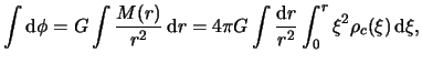
material. The integral for the gravitational potential produced by the
self-gravitating cloud is obtained from:
is the initial sound speed of the jet
material. The integral for the gravitational potential produced by the
self-gravitating cloud is obtained from:
where ![]() and
and ![]() represent the mass
and density of the cloud at a distance
represent the mass
and density of the cloud at a distance ![]() . Substitution of
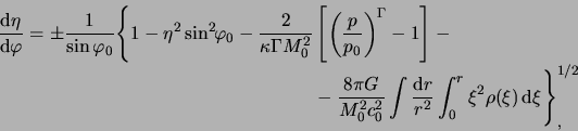
eqs.(17.8)-(17.10) into eq.(17.5) gives the
relation followed by the path of the jet as it expands:
. Substitution of
eqs.(17.8)-(17.10) into eq.(17.5) gives the
relation followed by the path of the jet as it expands:
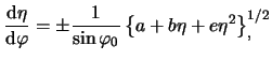
in which
![]() and
and ![]() is the initial
Mach number of the flow in the jet. The positive and negative signs
for the value of the derivative
is the initial
Mach number of the flow in the jet. The positive and negative signs
for the value of the derivative
![]() in eq.(17.11) have to be chosen with care. For example,
if we consider the case in which no gravity and no pressure gradients
are taken into account (i.e. last two terms on the right hand side of
eq.(17.11) are zero, which corresponds to a straight trajectory)
the derivative
in eq.(17.11) have to be chosen with care. For example,
if we consider the case in which no gravity and no pressure gradients
are taken into account (i.e. last two terms on the right hand side of
eq.(17.11) are zero, which corresponds to a straight trajectory)
the derivative
![]() for
for
![]() and vice versa. The equality
and vice versa. The equality
![]() corresponds to the point for which
a given fluid element in the jet reaches the y axis during its motion
in this particular case.
corresponds to the point for which
a given fluid element in the jet reaches the y axis during its motion
in this particular case.
In the limit of high initial supersonic motion (
![]() )
the third and fourth terms in the right hand side of eq.(17.11)
are important only when
)
the third and fourth terms in the right hand side of eq.(17.11)
are important only when
![]() and we can
simplify eq.(17.11) by making an expansion about this point.
Indeed, in general terms, if:
and we can
simplify eq.(17.11) by making an expansion about this point.
Indeed, in general terms, if:
are the expansions of the pressure and gravitational potential
respectively about
![]() , then eq.(17.11)
takes the form:
, then eq.(17.11)
takes the form:
 |
(17.13) |
|
in which:
| |
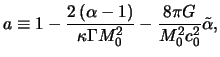 |
|
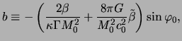 |
|
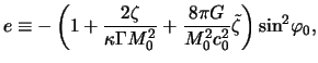 |
|
to second order in
![]() . For the cases
considered below, the general solution of eq.(17.14)
is (Gradshteyn & Ryzhik, 1994):
. For the cases
considered below, the general solution of eq.(17.14)
is (Gradshteyn & Ryzhik, 1994):
with
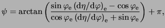
![]() . The angle
. The angle ![]() subtended between the velocity vector of the jet streamline with the
subtended between the velocity vector of the jet streamline with the ![]() coordinate axis on its way out of the cloud, the deflection
angle, can be calculated from the relation
coordinate axis on its way out of the cloud, the deflection
angle, can be calculated from the relation
![]() . In other words:
. In other words:
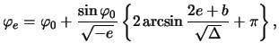
where the subindex ![]() labels the values of different
quantities at the position where the jet exits the cloud. The exit
azimuthal angle
labels the values of different
quantities at the position where the jet exits the cloud. The exit
azimuthal angle
![]() is given by:
is given by:
for not very strong deflections. The derivative
![]() is evaluated at
is evaluated at
![]() , with a negative choice of sign in eq.(17.11).
, with a negative choice of sign in eq.(17.11).
Sergio Mendoza Fri Apr 20, 2001

![$\displaystyle \eta=\frac{1}{2e} \left\{\sqrt{\Delta}\sin\left[\sqrt{-e}\left( \...
...{\sqrt{-e}} \arcsin \frac{ 2e + b }{\sqrt{\Delta}} \right) \right] -b \right\},$](img498.png)